Optimization Theory and Methods

WARNING

Optimization Problems

Mathematical Model

$$ \min f(\vec{x}),\vec{x}\in \vec{R^{n}} $$$$ \text{s.t.}{ \begin{cases} c_i(x)=0,& i \in E = {1,2,\cdots,l}\\ c_i(\vec{x})\ge 0,& i \in I = {l+1,\cdots,l+m}\\ \end{cases}} $$

where

• $\vec{x}=(x_1,x_2,\cdots,x_n)^T$ is called the decision variable vector
• $f(\vec{x})$ is the objective function
• s.t. means subject to, that is, the constraints

Classification

1. By time
   1. Static problems
   2. Dynamic problems
2. By constraints
   1. Constrained problems
   2. Unconstrained problems
3. By whether the objective and constraints are linear
   1. Linear programming
   2. Nonlinear programming
4. By whether the objective and constraints are convex
   1. Convex optimization problems
   2. Non-convex optimization problems

Quadratic Form Matrix

Quadratic form:

$$ \begin{align} f &=x_1^2-3x_3^2-4x_1x_2+x_2x_3\\ &=(x_1,x_2,x_3) \begin{bmatrix} 1 & -2 & 0\\ -2 & 0 & \frac{1}{2}\\ 0 & \frac{1}{2} & -3\\ \end{bmatrix} \begin{bmatrix} x_1\\ x_2\\ x_3\\ \end{bmatrix}\\ &= \vec{X^T} A \vec{X}\\ \end{align} $$

Quadratic form matrix:

$$ \begin{bmatrix} 1 & -2 & 0\\ -2 & 0 & \frac{1}{2}\\ 0 & \frac{1}{2} & -3\\ \end{bmatrix} $$

Hessian Matrix

Take a two-variable quadratic function as an example:

$$ \nabla^2 f(x_1,x_2)= \begin{bmatrix} \frac{\partial^2 f}{\partial x_1^2} & \frac{\partial^2 f}{\partial x_1 \partial x_2}\\ \frac{\partial^2 f}{\partial x_2 \partial x_1} & \frac{\partial^2 f}{\partial x_2^2}\\ \end{bmatrix} $$

Feasible Solutions

• Feasible solution: a solution satisfying all constraints.
• Feasible set (admissible set, feasible region): the set of all feasible solutions.
• Optimization problem: find the point in the feasible set at which the objective function attains its maximum or minimum.
• Stationary point: if $\nabla f(x_0)=0$, then $x_0$ is called a stationary point.
• Saddle point: if $x_0$ is a stationary point but not an extremum point, then it is called a saddle point.

Convex Sets

Definition

In the plane, if the line segment joining any two points inside a figure still lies entirely inside the figure, then the figure is called a convex set.

Properties

1. The intersection of convex sets is convex.
2. A scaled convex set is still convex.
3. The sum set of convex sets, not the union, is convex.
   • If $D_1,D_2$ are convex sets, then $D_1+D_2=\{z|z=x+y,x \in D_1,y \in D_2\}$ is convex.
4. A linear combination of convex sets is convex.

Common Convex Sets

1. The empty set
2. The whole Euclidean space $\vec{R^n}$
3. A hyperplane $H=\{x \in \vec{R^n} | a_1x_1+a_2x_2+\cdots +a_nx_n=b\}$
4. A half-space $H^+=\{x \in \vec{R^n} | a_1x_1+a_2x_2+\cdots +a_nx_n \ge b\}$

Convex Combination

Let $x_i \in \vec{R^n},i=1,2,\cdots ,k$, and let $\lambda_i \ge 0,\sum^k_{i=1}\lambda_i=1$. Then $x=\sum^k_{i=1}\lambda_ix_i$ is called a convex combination of $x_1,x_2,\cdots , x_k$.
Any finite convex combination of points in a convex set still belongs to that convex set.

Extreme Points

Let $D$ be a convex set and $x \in D$. If there do not exist two distinct points $y,z \in D$ and a real number $\alpha \in (0,1)$ such that $x=\alpha y+(1-\alpha)z$, then $x$ is called an extreme point of $D$.

In plain words: for a pentagon, the extreme points are its vertices; for a semicircle, the extreme points are the two endpoints of its diameter together with the top point on the arc.

Convex Functions

Definition

Let $f(x)$ be defined on a convex set. If for any two points $x_1,x_2$ in the convex set,

$$ f(\alpha x_1+(1-\alpha)x_2) \le \alpha f(x_1)+(1-\alpha)f(x_2) $$

then $f$ is called a convex function.
If the inequality is strict, $\lt$, then it is called a strictly convex function.

Criteria

1. If the Hessian matrix of a multivariable function is positive semidefinite, then the function is convex.
2. If the Hessian matrix is positive definite, then the function is strictly convex.
3. A multivariable linear function is convex on $\vec{R^n}$.

Convex Optimization Problems

Definition

An optimization problem in which the objective function and all constraint functions are convex functions.

• The feasible set of a convex optimization problem is convex.
• Any local optimum is also a global optimum.
• If the objective function is strictly convex, then the local optimum exists and is unique.

Linear Programming

Forms

Nonstandard Form

• Objective function: $\max z=\sum^{n}_{j=1}c_jx_j=CX$
• Coefficient matrix: $$ A= \begin{bmatrix} a_{11} & \cdots & a_{1n}\\ \vdots & \ddots & \vdots\\ a_{m1} & \cdots & a_{mn}\\ \end{bmatrix} =(P_1,P_2,\cdots,P_n) $$
• Resource vector: $b=\begin{bmatrix} b_1\\ \vdots \\ b_m\\ \end{bmatrix}$
• Decision variable vector: $X=(x_1,x_2,\cdots , x_n)^T$
• Constraints: $$ \begin{cases} \sum^{n}_{j=1}a_{ij}x_j=b_i,&i=1,2,\cdots,m\\ x_j \ge 0,& j=1,2,\cdots,n\\ \end{cases} $$ $$ \begin{cases} AX=b\\ X \ge \vec{0} \end{cases} $$

Standard Form

1. Convert a maximization problem into minimization
2. Slack variables: for $\le$ constraints, introduce slack variables to turn inequalities into equalities
3. Surplus variables: for $\ge$ constraints, introduce surplus variables to turn inequalities into equalities
4. Free variables: variables that may take arbitrary real values in practical problems, written as $x_i=x'-x''$

$$ \begin{cases} \min f(x_1,x_2,\cdots , x_n)\\ \text{s.t.} \begin{cases} h_j(x_1,x_2,\cdots,x_n)=0&(j=1,2,\cdots)\\ x_j \ge 0\\ \end{cases} \end{cases} $$

Basis Matrix

• Basis (basis matrix): a largest nonsingular submatrix of the coefficient matrix.
  • If the coefficient matrix $A$ is an $m \times n$ matrix with $rank(A)=m$, then any nonsingular $m \times m$ submatrix may serve as a basis matrix.
• Basic variables: the unknowns corresponding to the column vectors in the basis.
• Nonbasic variables: the unknowns that are not basic variables.
• Basic solution: the solution obtained by setting all nonbasic variables to zero.
• Nondegenerate basic solution: a basic solution in which the number of nonzero components equals the number of constraint equations. Otherwise it is a degenerate basic solution.
• Basic feasible solution: a basic solution satisfying the nonnegativity conditions in $\text{s.t.}$.
• Optimal basic feasible solution: among all basic feasible solutions, the one that gives the optimal objective value.

Properties of Linear Programming Solutions

1. The feasible set of a linear programming problem is convex.
2. If an optimal solution exists, it must be attained at a vertex of the feasible set.

Simplex Method

Reduced Costs

Each unknown corresponds to a reduced cost:

$$ \sigma_j=C^T_J \vec{P_j}-c_j=\sum^{m}_{i=1}c_ia_{ij}-c_j $$

• $C^T$ is the coefficient row of the objective function
• $C^T_J$ is the row of coefficients of the basic variables in the objective function
• $P_j$ denotes the $j$th column of matrix $A$
• $c_i$ denotes the coefficient of the $i$th basic variable in the objective function
• $c_j$ denotes the coefficient of the $j$th variable in the objective function and is unrelated to $c_i$

When all reduced costs are less than or equal to zero, the current basic feasible solution is optimal.

In general, the reduced costs of basic variables are zero.

Basis Transformation

Choosing the Basis Matrix

Prefer the identity matrix as the initial basis matrix. Compute the initial basic feasible solution and the reduced costs.

Constructing the Initial Simplex Tableau

	$P_1$	$P_2$	$\cdots$	$P_n$	$\vec{b}$
Coefficient matrix	$a_{11}$	$a_{12}$	$\cdots$	$a_{1n}$	$b_1$
	$a_{21}$	$a_{22}$	$\cdots$	$a_{2n}$	$b_2$
	$\vdots$	$\vdots$	$\ddots$	$\vdots$	$\vdots$
	$a_{m1}$	$a_{m2}$	$\cdots$	$a_{mn}$	$b_m$
Reduced costs	$\sigma_1$	$\sigma_2$	$\cdots$	$\sigma_n$	Optimal value

Selecting an Entering Column

If a reduced cost is greater than zero, then the corresponding column has improving potential. Choose this column as the entering column $P_j$, and the corresponding variable $x_j$ is the entering variable.

Selecting the Pivot Element

Among the positive entries $a_{ij}$ in the entering column, divide the corresponding entry of $b$ by each such element and choose the smallest ratio. The corresponding element $a_{ij}$ is the pivot.
If a reduced cost is greater than zero but all entries in that column are negative, then the linear program has no optimal solution.

Elementary Row Operations

Transform the pivot into 1 and all other entries in that column into 0.
Geometric meaning: moving to another vertex of the feasible region.

Leaving Column

Select the new basis matrix according to the updated coefficient matrix. Compared with the old basis, the replaced column is the leaving column, and its corresponding variable is the leaving variable.
Then recompute the reduced costs and form the new simplex tableau.

A New Basis Transformation

If the reduced-cost row changes and new positive reduced costs appear, choose the corresponding column as the new entering column, select a pivot, and perform elementary row operations again.

Result

When all reduced costs are less than or equal to zero, the entries of $\vec{b}$ are the values of the basic variables, while the nonbasic variables are set to 0. Together these form the optimal solution, and substituting them into the objective function gives the minimum value.

Conditions for Applying the Simplex Method

1. All elements in the nonhomogeneous term are nonnegative.
2. A feasible solution exists.
3. The sum of products of slack variables and nonbasic variables is zero.
4. The problem is a linear programming problem on a convex feasible region.
5. The feasible solution set is finite.

Artificial Variable Method

When the coefficient matrix does not contain an identity matrix, one usually introduces artificial variables to construct one artificially.

Suppose the constraints of the linear programming problem are $\sum^{n}_{j=1}a_{ij}=b_i(i=1,2,\cdots ,m)$. Add artificial variables $x_{n+1},x_{n+2},\cdots,x_{n+m}$ to each constraint and use them as the basic variables, so that they form an identity matrix and all other variables are zero. In this way we obtain an initial feasible solution $x^{(0)}=(0,0,\cdots,0,b_1,b_2,\cdots,b_m)^T$.
Starting from this point, carry out basis transformations to obtain an optimal solution without nonzero artificial variables.

If all reduced costs are negative but nonzero artificial variables still remain, then the original problem has no feasible solution.

Big-M Method

For a minimization problem, after introducing artificial variables into the constraints, assign the coefficient $M$ to the artificial variables in the objective function, where $M \in \vec{R^+}$.
To obtain the minimum objective value, one keeps carrying out basis transformations until the artificial variables become zero. For a maximization problem, $M \in \vec{R^-}$.

Degenerate Cases

If the simplex method falls into cycling while the problem does have an optimal solution, the following methods may be used to avoid cycling.

Perturbation Method

Revised Simplex Method

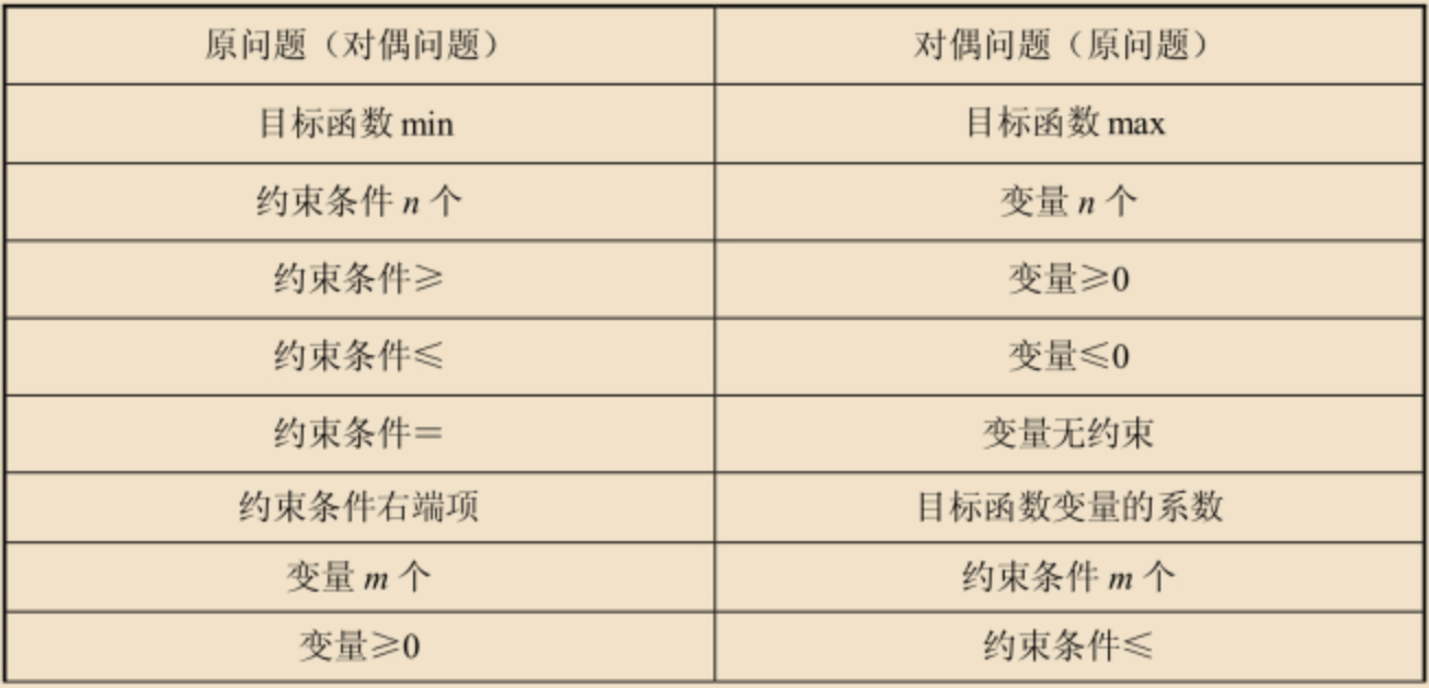
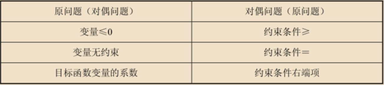
Duality Theory of Linear Programming

Forms of the Dual Problem

Symmetric Form

Primal problem

$$ \begin{cases} \min f=\vec{c^T}\vec{x}\\ \text{s.t.} \begin{cases} \vec{A}\vec{x} \ge \vec{b}\\ \vec{x} \ge \vec{0} \end{cases} \end{cases} $$

Dual problem

$$ \begin{cases} \max w=\vec{b^T}\vec{y}\\ \text{s.t.} \begin{cases} \vec{A^T}\vec{y} \le \vec{c}\\ \vec{y} \ge \vec{0}\\ \end{cases} \end{cases} $$

Correspondence:

• (1) The number of constraints in the primal problem equals the number of variables in its dual.
• (2) The coefficients of the primal objective function become the right-hand-side constants of the dual constraints.
• (3) If the primal objective is minimization, then the dual objective is maximization.
• (4) If the primal constraints are of type “$\ge$”, then the dual constraints are of type “$\le$”.

Asymmetric Form

Primal problem

$$ \begin{cases} \min f=\vec{c^T}\vec{x}\\ \text{s.t.} \begin{cases} \vec{A}\vec{x} = \vec{b}\\ \vec{x} \ge \vec{0} \end{cases} \end{cases} $$

Dual problem

$$ \begin{cases} \max w=\vec{b^T}\vec{y}\\ \text{s.t.} \begin{cases} \vec{A^T}\vec{y} \le \vec{c}\\ \vec{y} \text{ is unrestricted} \end{cases} \end{cases} $$

General Case

If the primal problem contains a mixture of $\le,\ge,=$ constraints, first introduce slack and surplus variables so that all constraints become equalities, and then construct the dual using the asymmetric form.

Dual Simplex Method

• Simplex method: first ensure $\vec{b} \ge 0$, then iterate based on reduced costs $\le 0$.
• Dual simplex method: first ensure reduced costs $\le 0$, then iterate based on $\vec{b} \ge 0$.

Ensuring Reduced Costs $\le 0$

Choosing the Leaving Variable

If there exists a negative $b_i \lt 0$, then the row containing the smallest $\min b_i$ is chosen as the leaving row, and the corresponding variable is the leaving variable.

Choosing the Entering Variable

Divide each reduced cost by the negative coefficient in the leaving row, that is, $a_{ij} \lt 0$. The column corresponding to the smallest resulting value is chosen as the entering column, and the corresponding variable is the entering variable.

Row Operations

Use elementary row operations to transform the entering column into one that matches the basis matrix, that is, an identity column. At this point $\vec{b}$ changes as well.
Then recompute the reduced costs and ensure that they remain less than or equal to zero.

A New Basis Transformation

If there is still a negative value $b_i \lt 0$, choose the smallest $\min b_i$ and perform another basis transformation.

Result

When all $b_i \ge 0$, the vector $\vec{b}$ gives the optimal values of the basic variables, while the nonbasic variables are 0.
Substitute them into the objective function to obtain the optimal value, whether maximum or minimum.

Sensitivity Analysis